RELATED |
By the 1989 Gordon Bell Prize Committee
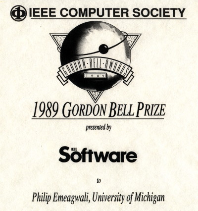
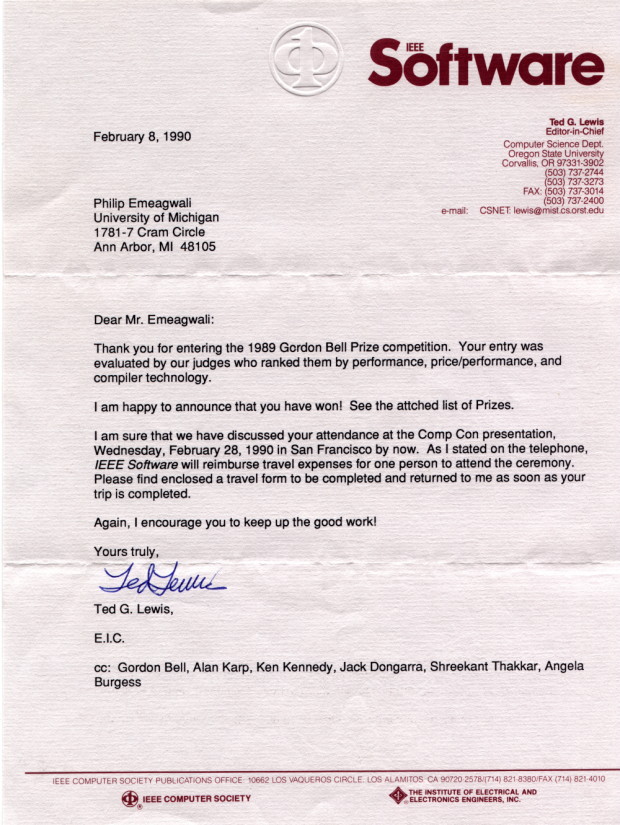
The Gordon Bell Prize recognizes significant achievements in the application of supercomputers to scientific and engineering problems. . . . We awarded the price/performance prize to Philip Emeagwali of the Civil Engineering Department and Scientific Computing Program at the University of Michigan at Ann Arbor. He also used a CM-2 to solve an oil-reservoir-modeling problem. . . .
Connection MachineA little background on the CM-2's architecture is helpful to understand how this year's winners achieved such outstanding performance.The Connection Machine is a massively parallel, single-instruction, multiple-data machine, in which all processors execute the same instruction at each machine cycle. It handles conditional execution by providing each processor with a mask bit --- a processor executes and instruction only if its mask bits is on. The CM-2 has up to 65,536 one-bit processors and 4,096 nodes, each containing 16 processors. Each processor has a local memory of 32 Kbytes. For floating-point computations, groups of 32 processors talk to a single floating-point processor capable of a 14-Mflop computation rate. Thus, if all 2,048 floating-point processors can be kept busy, the CM-2 can compute at 28 Gflops. A Data Vault made up of 42 hard-disk drives, connected directly to the processors, provides high-speed I/O. There is no global memory, so the processors must exchange data explicitly. They communicate over a 12-dimensional hypercube, so each chip has 12 neighbors. The CM-2 provides two communication mechanisms: the North-East-West-South network, which lets nearest neighbors communicate in a 2D grid, and a router for more general communications. In addition, there are library routines for commonly used discretizations of partial differential equations, which makes the CM-2 particularly efficient at running finite-difference methods. To program a machine like the CM-2, you follow the basic data-parallelism concept: You divide the problem into an extremely large number of pieces that need the exact same sequence of operations performed. For example, to add two matrices, you assign one element of each of the two input matrices and the output matrix to each processor, and issue load, add, and store instructions to all processors. If the matrix is no larger than order 256 (256 times 256, or 65,536), adding these two matrices will take exactly as long as adding any single element pair. You can handle very large problems with virtual processors, which let you treat the machine as if it had many more processors. For example, with a virtual-processor ratio of 4:1, you write the program as if you had $262,144$ processors, each with 8 Kbytes of memory. Each virtual processor is time-sliced on the physical processors, so adding two matrices of order 512 will take four times longer than two order 256 matrices. But virtual processors are more than a programming convenience. Because the virtual processors assigned to a single physical processor share a common memory, communications among them is particularly fast. You run the CM-2 from a front-end processor: a Digital Equipment Corp. VAX, a Sun 4 workstation, or a Symbolics Lisp machine. You do all application development on the front end. The front end executes any instructions dealing with single numbers: the CM-2 executes any instructions that refer to parallel variables. You program the Connection Machine in Paris (a machine language), Lisp*, C*, or Fortran 8x. Both this year's winners programmed in Fortran 8x. TMC's [Thinking Machines Corporation] version of Fortran 8x does all the work on the Connection Machine and all scalar work on the front end. . . . Finding oil is expensive. Each exploratory well costs millions of dollars, and it is not unusual to to sink many wells before oil is found. There is, therefore, a great incentive to reduce the number of dry wells.
Today's engineers use several distinct steps to find new oil fields. First,
they collect data in the field using an array of microphones, either
placed on the ground or towed behind a boat. They generate sound waves,
which reflect off subterranean structures and are detected by the microphones.
The data is cleaned up and filtered to remove the effects of noise and
multiple reflections.
Model building, the step that consumes most of the CPU time, is an inverse problem, solved by repeatedly modeling the sound-wave propagation through different assumed velocity distributions. Today, the most common algorithms used in the oil industry is the finite-difference methods applied to the sound-wave equation, which involves second derivatives of the pressure with respect to the two spae variables and time. The Mobil/TMC team used this approach in its winning entry. . . .
Once you find the oil, you want to maximize the amount you pump out
of the ground. The amount of oil you recover can be reduced drastically
if you do things wrong. For example, many oil fields are surrounded
by water, and water is much more mobile in the rock. If you pump
the oil too fast, the surrounding water may intrude into the oil field.
You'll end up pumping lots more water than oil, and you'll lose
the remaining oil forever.
The amount of money at stake is staggering. For example, you can typically expect to recover 10 percent of a field's oil. If you can improve your production schedule to get just 1 percent more oil, you will increase your yield by $400 million (at $20 per barrel in a 20-billion-barrel field). Maybe that's why 10 percent of all supercomputers are used for reservoir modeling.
EquationsReservoir-modeling equations are extremely challenging. The simulations must follow many constituents, like water, methane, and liquid hydrocarbons; the equations are highly nonlinear, resulting in steep discontinuities in the solution; the underlying geometry is complicated by irregularities in the rock's boundaries and flow properties; and realistic results normally requires following the flow in three dimensions.Reservoir modeling equations are similar to other fluid-flow models, but they do have some unique properties. Some equations balance the forces due to pressure, gravity. advection, and drag due to viscosity on the components being modeled. Other algebraic relations, called state equations, specify things like the volume of a given water mass at a specified temperature and pressure and a constituent's viscosity under specified conditions. They are also many prespecified quantities like fluid composition and the rock's properties. These equations are nonlinear: The gases' vapor pressure is determined by the total pressure, which in turn depends on flow velocity; flow velocity depends on rock and pressure and rock properties, which depends on saturation. (Saturation describes fluid composition: If the fluid is 10-percent water and 90-percent oil, its water saturation is 0.1 and its oil saturation is 0.9) Many of these nonlinear lead to near discontinuities in the flow. Numerical solutions do not do well in the presence of discontinuities in the flow, so you must do something to get accurate solutions in a reasonable amount of time. The most common approach is to add a small amount of artificial viscosity to the physical viscosity, which smears the discontinuities over several grid points without affecting the solution too much.
Time DimensionTo advance the equations in time, you can use explicit or implicit methods. Explicit methods are computationally simple: You express the unknowns at the new time in terms of the unknown at the old time and compute the new values directly. The disadvantage of explicit methods is that the discretizations is stable only for extremely small time steps --- seconds for reservoir modeling. Because you need to model the reservoir over decades, explicit methods have been considered impractical. Implicit methods involve more computation: You express the unknows at the new time in terms of both the old values and the new values and then you solve these nonlinear, implicit equations iteratively.Most commercial reservoir simulators use a combination of these methods called implicit pressure, explicit saturation. These methods solve the saturation equation for each constituent explicitly and the more unstable pressure equation implicitly. In practice, you can simplify the saturation equations by ignoring convective terms. This assumption is safe because these terms are small relative to the other terms. What is left is an equation that says the force on the fluid is proportional to the gradient. You can simplify the pressure equations by assuming that velocity depends linearly on viscous force, which is accurate for these high-viscosity problems. This leaves a parabolic equation for pressure instead of the more difficult hyperbolic equation you began with. The pressure equations are solved implicitly, using the pressure gradient to determine the velocity, and then the saturations for each constituent are advanced explicitly to the new time. The iterative methods used to solve the pressure equations involve solving large systems of linear equations at each iteration of the nonlinear solution. These linear equations are much too large to solve with a direct method like Gauss elimination, so they are also solved by iterative methods. Unfortunately, iterative methods work best for symmetrical, positive, definite matrices --- which these systems are not. Thus, today's reservoir simulators differ primarily in how well they solve very large linear systems.
SolutionSometimes you need to step back from a problem to see a solution. Emeagwali did just that. He returned to the original pressure equation. Solving the full system, although more daunting, carries certain advantages. You can compute velocities directly instead of from a numerical derivative of the pressure, so they are more accurate. You can use more general boundary conditions. You can achieve a higher order of accuracy when you discretize the equations on nonuniform grids. Finally, you don't need to change the equations when the flow becomes turbulent.The only problem is to make it work with reasonable time steps. Although implicit discretization allows large time steps, the CM-2 is much more efficient with explicit methods, which require much smaller time steps. Emeagwali's solution was direct --- he simply multiplied these small terms by a large number. His numerical experiments showed virtually no change in the computed results with multipliers as large as 1,000, but he could increase his time steps by a factor of 30. In a way, this artificially large inertial term is analogous to the artificially large viscosity that smoothes discontinuities. As long as the corresponding terms are kept small relative to the other terms, they can be increased without drastically affecting the results. Emeagwali's entry described two problems. One was a 2D model that followed the flow of pure oil through a grid of 8 million points. The other, more realistic, 3D model followed the flow of three phases --- oil, water, and gas --- through a grid of 1 million points. The size of the 3D simulation was limited solely by the CM-2's memory.
These are very large simulations. Commercial simulators
typically use a few hundred thousand grid points. Due to limited
memory, Emeagwali's 3D model solved for only 18 million unknowns
per time step compared to 24 million in the 2D model.
Both models took about one-sixth of a second of real time per time
step, and both were followed for several hundred time steps. These times
translate into 3.1 Gflops for the 2D model and 2.9 Gflops for
the 3D model.
Reported by Jack Dongarra, Alan H. Karp, Ken Kennedy and David Kuck --- the 1989 Gordon Bell Prize judges for the Institute for Electrical and Electronics Engineers --- in the May 1990 issue of IEEE Software.


Click on emeagwali.com for more information.
|